Book of AOS

AOS Storage

» Download this section as PDF (opens in a new tab/window)

Nutanix AOS storage is the scale-out storage technology that appears to the hypervisor like any centralized storage array, however all of the I/Os are handled locally to provide the highest performance.  More detail on how these nodes form a distributed system can be found in the next section.

Data Structure

Nutanix AOS storage is composed of the following high-level struct:

Storage Pool

• Key Role: Group of physical devices
• Description: A storage pool is a group of physical storage devices including PCIe SSD, SSD, and HDD devices for the cluster. The storage pool can span multiple Nutanix nodes and is expanded as the cluster scales. In most configurations, only a single storage pool is leveraged.

Container

• Key Role: Group of VMs/files
• Description: A container is a logical segmentation of the Storage Pool and contains a group of VM or files (vDisks). Some configuration options (e.g., RF) are configured at the container level, however are applied at the individual VM/file level. Containers typically have a 1 to 1 mapping with a datastore (in the case of NFS/SMB).

vDisk

• Key Role: vDisk
• Description: A vDisk is any file over 512KB on AOS including .vmdks and VM hard disks. vDisks are logically composed of vBlocks which make up the ‘block map.’

The following figure shows how these map between AOS and the hypervisor:

High-level Filesystem Breakdown

vBlock

• Key Role: 1MB chunk of vDisk address space
• Description: A vBlock is a 1MB chunk of virtual address space composing a vDisk. For example, a vDisk of 100MB will have 100 x 1MB vBlocks, vBlock 0 would be for 0-1MB, vBlock 1 would be from 1-2MB, and so forth. These vBlocks map to extents which are stored as files on disk as extent groups.

Extent

• Key Role: Logically contiguous data
• Description: An extent is a 1MB piece of logically contiguous data which consists of n number of contiguous blocks (varies depending on guest OS block size). Extents are written/read/modified on a sub-extent basis (aka slice) for granularity and efficiency. An extent’s slice may be trimmed when moving into the cache depending on the amount of data being read/cached.

Extent Group

• Key Role: Physically contiguous stored data
• Description: An extent group is a 1MB or 4MB piece of physically contiguous stored data. This data is stored as a file on the storage device owned by the CVM. Extents are dynamically distributed among extent groups to provide data striping across nodes/disks to improve performance. NOTE: as of 4.0, extent groups can now be either 1MB or 4MB depending on deduplication.

The following figure shows how these structs relate between the various file systems: 

Low-level Filesystem Breakdown

Here is another graphical representation of how these units are related:

Graphical Filesystem Breakdown

I/O Path and Cache

For a visual explanation, you can watch the following video: LINK

The typical hyperconverged storage I/O path can be characterized into the following core layers:

1. Guest OS (UVM) to virtual disk(s)
   • This remains unchanged with Nutanix. Depending on the hypervisor the guest OS will use a device driver to talk to a virtual disk device. Depending on the hypervisor this could be virtio-scsi (AHV), pv-scsi (ESXi), etc. The virtual disks will also vary based upon the hypervisor (e.g. vmdk, vhd, etc.)
2. Hypervisor to AOS (via CVM)
   • Communication between the hypervisor and Nutanix occurs via standard storage protocols (e.g. iSCSI, NFS, SMBv3) over the local interface of the CVM and hypervisor. At this point all communication has been local to the host (there are scenarios where I/O will be remote (e.g. local CVM down, etc.).
3. Nutanix I/O path
   • This is all transparent to the hypervisor and UVMs and it native to the Nutanix platform.

The following image shows a high-level overview of these layers:

High-level I/O Path - Traditional

Communication and I/O

Within the CVM the Stargate process is responsible for handling all storage I/O requests and interaction with other CVMs / physical devices. Storage device controllers are passed through directly to the CVM so all storage I/O bypasses the hypervisor.

The following image shows a high-level overview of the traditional I/O path:

High-level I/O Path

Nutanix BlockStore (shipped in AOS 5.18) is an AOS capability which creates an extensible filesystem and block management layer all handled in user space. This eliminates the filesystem from the devices and removes the invoking of any filesystem kernel driver. The introduction of newer storage media (e.g. NVMe), devices now come with user space libraries to handle device I/O directly (e.g. SPDK) eliminating the need to make any system calls (context switches). With the combination of BlockStore + SPDK all Stargate device interaction has moved into user space eliminating any context switching or kernel driver invocation.

Stargate - Device I/O Path

The following image shows a high-level overview of the updated I/O path with BlockStore + SPDK:

High-level I/O Path - BlockStore

To perform data replication the CVMs communicate over the network. With the default stack this will invoke kernel level drivers to do so.

However, with RDMA these NICs are passed through to the CVM, bypassing the hypervisor and reducing interrupts. Also, within the CVM all network traffic using RDMA only uses a kernel level driver for the control path, then all actual data I/O is done in user-space without any context switches.

The following image shows a high-level overview of the I/O path with RDMA:

High-level I/O Path - RDMA

To summarize, the following enhancements optimize with the following:

1. PCI passthrough bypasses the hypervisor for device I/O
2. SPDK + Blockstore eliminates kernel storage driver interactions and moves them to user-space
3. RDMA bypasses the hypervisor and all data transfer is done in CVM user-space

Stargate I/O Logic

Within the CVM the Stargate process is responsible for handling all I/O coming from user VMs (UVMs) and persistence (RF, etc.). When a write request comes to Stargate, there is a write characterizer which will determine if the write gets persisted to the OpLog for bursty random writes, or to Extent Store for sustained random and sequential writes. Read requests are satisfied from Oplog or Extent Store depending on where the data is residing when it is requested.

The Nutanix I/O path is composed of the following high-level components:

AOS I/O Path

*As of AOS 5.10, the Autonomous Extent Store (AES) can be used to handle sustained random workloads when requisite conditions are met.

^:

1. In all-flash node configurations (All NVMe SSD, All SATA/SAS SSD, NVMe+SATA/SAS SSD) the Extent Store will only consist of SSD devices and no tier ILM will occur as only a single flash tier exists.
2. In cases where Optane is used (e.g. Intel Optane + NVMe/SATA SSD) the highest performance media will be Tier 0 and the lower performance media will be Tier 1.
3. For hybrid scenarios with flash and HDD, the flash would be Tier 0 with HDD being Tier 1.
4. OpLog is always on SSDs in Hybrid Clusters and on both Optane and NVMe SSDs in Optane+NVMe clusters.
5. Data is moved between tiers by Intelligent Lifecycle Management (ILM) based on access patterns.

OpLog

• Key Role: Persistent write buffer
• Description: The OpLog is similar to a filesystem journal and is built as a staging area to handle bursts of random writes, coalesce them, and then sequentially drain the data to the extent store. Upon a write, the OpLog is synchronously replicated to another n number of CVM’s OpLog before the write is acknowledged for data availability purposes. All CVM OpLogs partake in the replication and are dynamically chosen based upon load. The OpLog is stored on the SSD tier on the CVM to provide extremely fast write I/O performance, especially for random I/O workloads. All SSD devices participate and handle a portion of OpLog storage. For sequential workloads, the OpLog is bypassed and the writes go directly to the extent store. If data is currently sitting in the OpLog and has not been drained, all read requests will be directly fulfilled from the OpLog until they have been drained, where they would then be served by the extent store/unified cache. For containers where fingerprinting (aka Dedupe) has been enabled, all write I/Os will be fingerprinted using a hashing scheme allowing them to be deduplicated based upon fingerprint in the unified cache.

Extent Store

• Key Role: Persistent data storage
• Description: The Extent Store is the persistent bulk storage of AOS and spans all device tiers (Optane SSD, PCIe SSD, SATA SSD, HDD) and is extensible to facilitate additional devices/tiers. Data entering the extent store is either being A) drained from the OpLog or B) is sequential/sustained in nature and has bypassed the OpLog directly. Nutanix ILM will determine tier placement dynamically based upon I/O patterns, number of accesses of data and weight given to individual tiers and will move data between tiers.

Autonomous Extent Store (AES)

• Key Role: Persistent data storage
• Description: The Autonomous Extent Store (AES) is a new method for writing / storing data in the Extent Store introduced in AOS 5.10. It leverages a mix of primarily local + global metadata (more detail in the ‘Scalable Metadata’ section following) allowing for much more efficient sustained performance due to metadata locality. For sustained random write workloads, these will bypass the OpLog and be written directly to the Extent Store using AES. For bursty random workloads these will take the typical OpLog I/O path then drain to the Extent Store using AES where possible. As of AOS 5.20 (LTS), AES is enabled by default for new containers on All Flash Clusters and as of AOS 6.1 (STS) if requirements are met, AES is enabled on new containers created on Hybrid(SSD+HDD) Clusters.

Unified Cache

• Key Role: Dynamic read cache
• Description: The Unified Cache is a read cache which is used for data, metadata and deduplication and stored in the CVM’s memory. Upon a read request of data not in the cache (or based upon a particular fingerprint), the data will be read from the extent store and will also be placed into the single-touch pool of the Unified Cache which completely sits in memory, where it will use LRU (least recently used) until it is evicted from the cache. Any subsequent read request will “move” (no data is actually moved, just cache metadata) the data into the multi-touch pool. Any read request for data in the multi-touch pool will cause the data to go to the peak of the multi-touch pool where it will be given a new LRU counter. Cache size can be calculated using the following formula: ((CVM Memory - 12 GB) * 0.45). For example a 32GB CVM would have the following cache size: ((32 - 12)*0.45) == 9GB.

The following figure shows a high-level overview of the Unified Cache:

AOS Unified Cache

Single vDisk Sharding

AOS was designed and architected to deliver performance for applications at scale. Inside Stargate, I/O is processed by threads for every vdisk created by something called vdisk controller. Every vdisk gets its own vdisk controller inside Stargate responsible for I/O for that vdisk. The expectation was that workloads and applications would have multiple vdisks each having its own vdisk controller thread capable of driving high performance the system is capable of delivering.

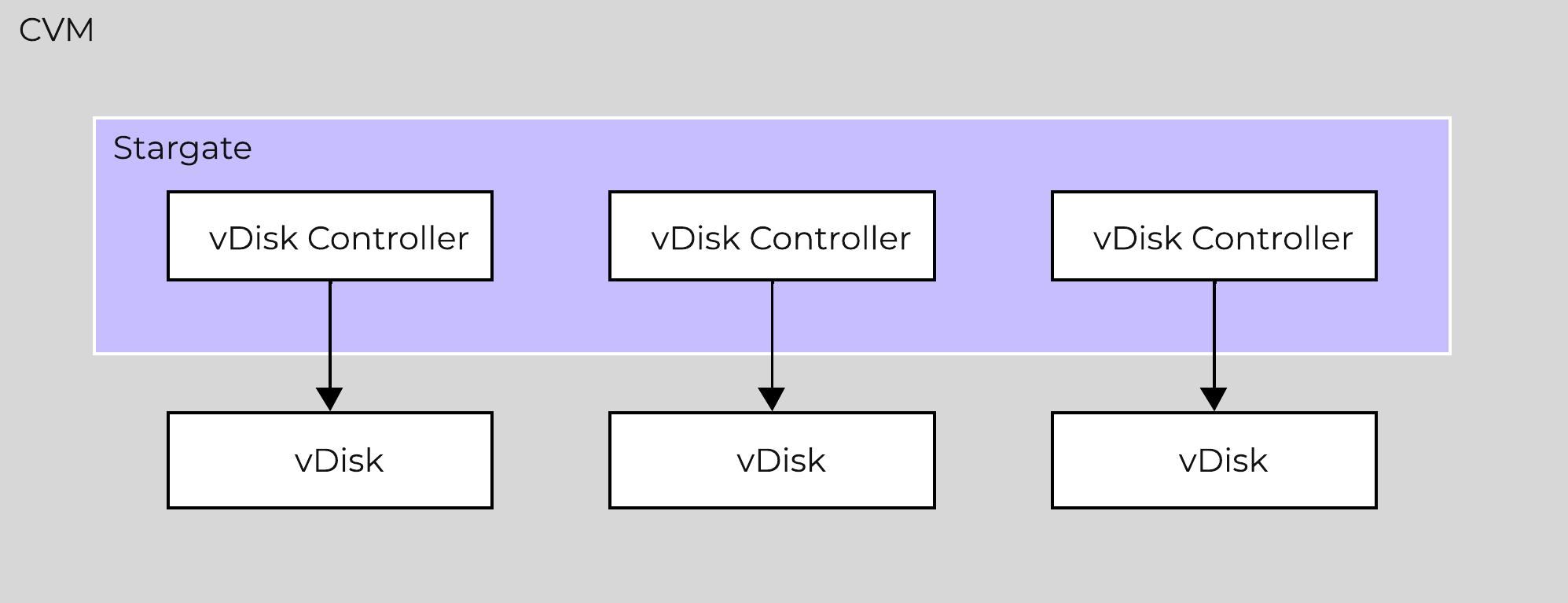
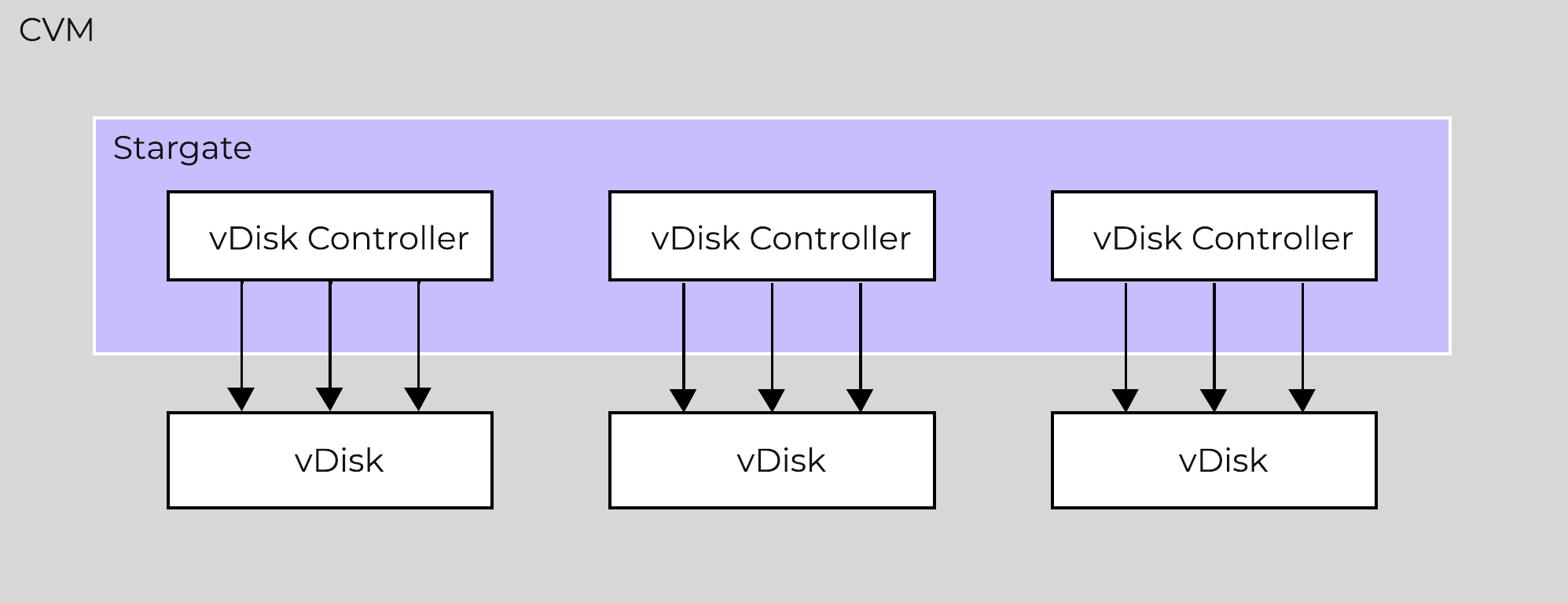
This architecture worked well except in cases of traditional applications and workloads that had VMs with single large vdisk. These VMs were not able to leverage the capabilities of AOS to its fullest. As of AOS 6.1, enhancement was done to vdisk controller such that requests to a single vdisk are now distributed to multiple vdisk controllers by creating shards of the controller each having its own thread. I/O distribution to multiple controllers is done by a primary controller so for external interaction this still looks like a single vdisk. This results in effectively sharding the single vdisk making it multi-threaded. This enhancement alongwith other technologies talked above like Blockstore, AES allows AOS to deliver consistent high performance at scale even for traditional applications that use a single vdisk.

Scalable Metadata

For a visual explanation, you can watch the following YouTube video: Tech TopX by Nutanix University: Scalable Metadata

Metadata is at the core of any intelligent system and is even more critical for any filesystem or storage array. For those unsure about the term ‘metadata’; essentially metadata is ‘data about data’. In terms of AOS, there are a few key principles that are critical for its success:

• Must be right 100% of the time (known as “strictly consistent”)
• Must be ACID compliant
• Must have unlimited scalability
• Must not have any bottlenecks at any scale (must be linearly scalable)

As of AOS 5.10 metadata is broken into two areas: global vs. local metadata (prior all metadata was global). The motivation for this is to optimize for “metadata locality” and limit the network traffic on the system for metadata lookups.

The basis for this change is that not all data needs to be global. For example, every CVM doesn’t need to know which physical disk a particular extent sits on, they just need to know which node holds that data, and only that node needs to know which disk has the data.

By doing this we can limit the amount of metadata stored by the system (eliminate metadata RF for local only data), and optimize for “metadata locality.”

The following image shows the differentiation between global vs. local metadata:

Global vs. Local Metadata

Local Metadata

• Description:
  • Local metadata store per CVM containing information only needed by the local node. This is leveraged by the Autonomous Extent Store (AES) introduced in 5.10.
• Storage Mechanism:
  • AES DB (based on Rocksdb)
• Types of data stored:
  • Physical extent / extent group placement (e.g. egroup to disk mappings), etc.

Global Metadata

• Description:
  • Metadata that is globally available to any CVM and sharded across CVMs in the cluster. All metadata prior to 5.10.
• Storage Mechanism:
  • Medusa Store (based on Cassandra)
• Types of data stored:
  • vDisk block maps, extent to node mappings, time series stats, configurations, etc.

The section below covers how global metadata is managed:

As mentioned in the architecture section above, AOS utilizes a “ring-like” structure as a key-value store which stores essential global metadata as well as other platform data (e.g., stats, etc.). In order to ensure global metadata availability and redundancy a replication factor (RF) is utilized among an odd amount of nodes (e.g., 3, 5, etc.). Upon a global metadata write or update, the row is written to a node in the ring that owns that key and then replicated to n number of peers (where n is dependent on cluster size).  A majority of nodes must agree before anything is committed, which is enforced using the Paxos algorithm.  This ensures strict consistency for all data and global metadata stored as part of the platform.

The following figure shows an example of a global metadata insert/update for a 4 node cluster:

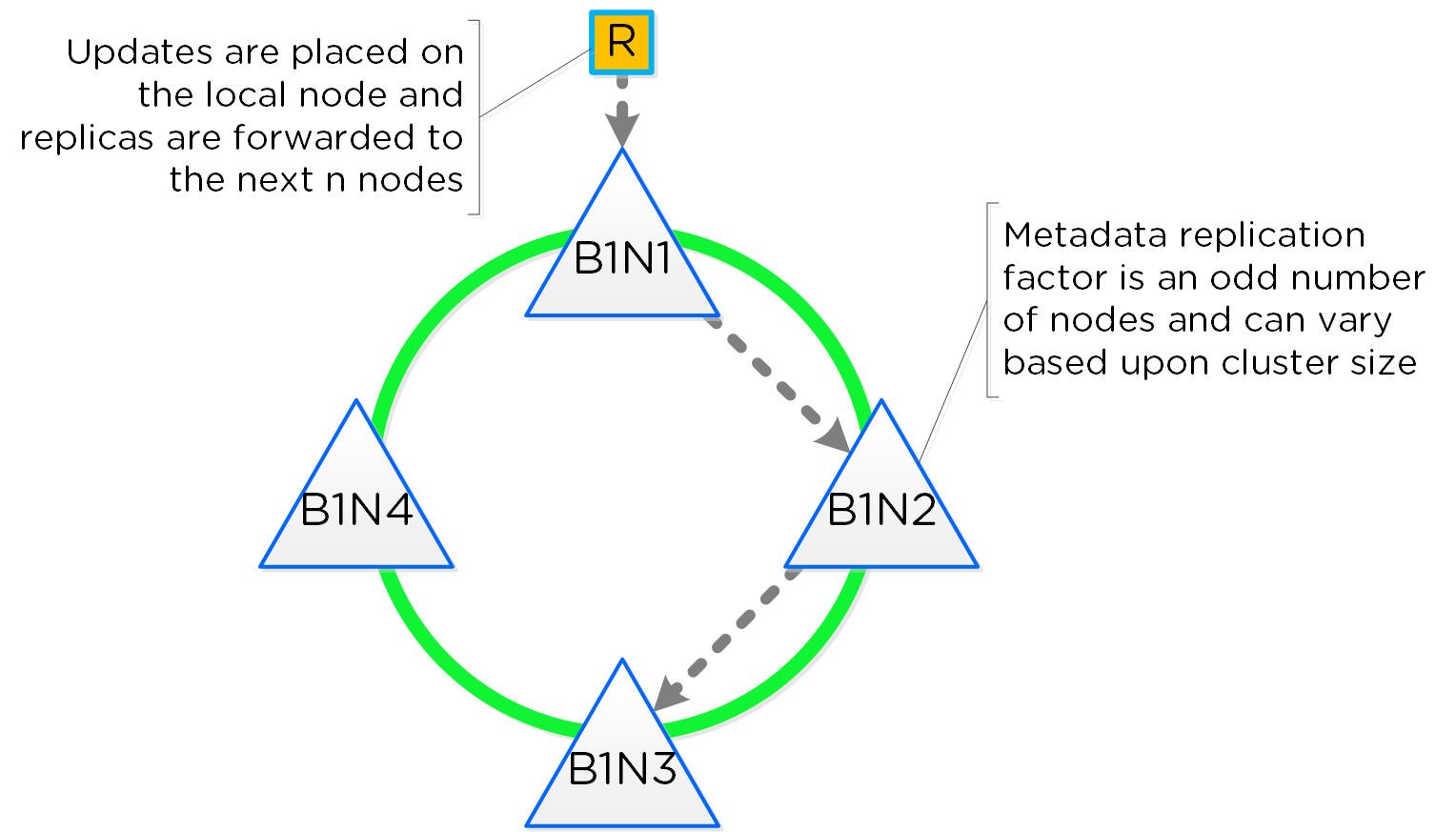Cassandra Ring Structure

Performance at scale is also another important struct for AOS global metadata.  Contrary to traditional dual-controller or “leader/worker” models, each Nutanix node is responsible for a subset of the overall platform’s metadata.  This eliminates the traditional bottlenecks by allowing global metadata to be served and manipulated by all nodes in the cluster.  A consistent hashing scheme is utilized for key partitioning to minimize the redistribution of keys during cluster size modifications (also known as “add/remove node”). When the cluster scales (e.g., from 4 to 8 nodes), the nodes are inserted throughout the ring between nodes for “block awareness” and reliability.

The following figure shows an example of the global metadata “ring” and how it scales:

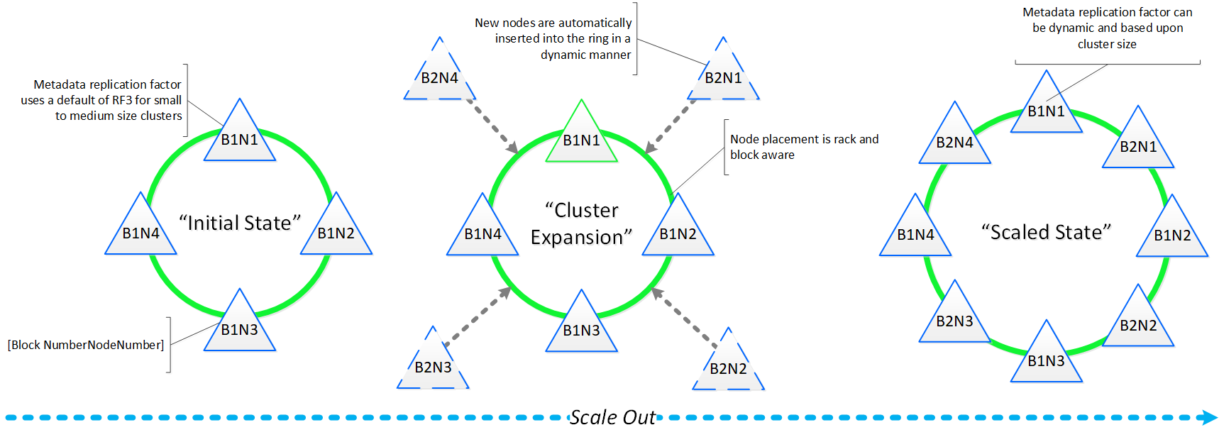Cassandra Scale Out

Data Protection

For a visual explanation, you can watch the following video: LINK

The Nutanix platform currently uses a resiliency factor, also known as a replication factor (RF), and checksum to ensure data redundancy and availability in the case of a node or disk failure or corruption.  As explained above, the OpLog acts as a staging area to absorb incoming writes onto a low-latency SSD tier.  Upon being written to the local OpLog, the data is synchronously replicated to another one or two Nutanix CVM’s OpLog (dependent on RF) before being acknowledged (Ack) as a successful write to the host.  This ensures that the data exists in at least two or three independent locations and is fault tolerant. NOTE: For RF3, a minimum of 5 nodes is required since metadata will be RF5. 

OpLog peers are chosen for every episode (1GB of vDisk data) and all nodes actively participate. Multiple factors play into which peers are chosen (e.g. response time, business, capacity utilization, etc). This eliminates any fragmentation and ensures every CVM/OpLog can be used concurrently.

Data RF is configured via Prism and is done at the container level. All nodes participate in OpLog replication to eliminate any “hot nodes”, ensuring linear performance at scale.  While the data is being written, a checksum is computed and stored as part of its metadata. Data is then asynchronously drained to the extent store where the RF is implicitly maintained.  In the case of a node or disk failure, the data is then re-replicated among all nodes in the cluster to maintain the RF.  Any time the data is read, the checksum is computed to ensure the data is valid.  In the event where the checksum and data don’t match, the replica of the data will be read and will replace the non-valid copy.

Data is also consistently monitored to ensure integrity even when active I/O isn’t occurring. Stargate’s scrubber operation will consistently scan through extent groups and perform checksum validation when disks aren’t heavily utilized. This protects against things like bit rot or corrupted sectors.

The following figure shows an example of what this logically looks like: 

AOS Data Protection

Availability Domains

For a visual explanation, you can watch the following video: LINK

Availability Domains (aka node/block/rack awareness) is a key struct for distributed systems to abide by for determining component and data placement. Nutanix refers to a “block” as the chassis which contains either one, two, or four server “nodes” and a “rack” as a physical unit containing one or more “block”. NOTE: A minimum of 3 blocks must be utilized for block awareness to be activated, otherwise node awareness will be used.

Nutanix currently supports the following levels or awareness:

• Disk (always)
• Node (always)
• Block (as of AOS 4.5)
• Rack (as of AOS 5.9)

It is recommended to utilize uniformly populated blocks / racks to ensure the awareness is enabled and no imbalance is possible. Common scenarios and the awareness level utilized can be found at the bottom of this section. The 3-block requirement is due to ensure quorum. For example, a 3450 would be a block which holds 4 nodes. The reason for distributing roles or data across blocks is to ensure if a block fails or needs maintenance the system can continue to run without interruption. NOTE: Within a block, the redundant PSU and fans are the only shared components.

NOTE: Rack awareness requires the administrator to define “racks” in which the blocks are placed.

The following shows how this is configured in Prism:

Rack Configuration

Awareness can be broken into a few key focus areas:

• Data (The VM data)
• Metadata (Cassandra)
• Configuration Data (Zookeeper)

Data

With AOS, data replicas will be written to other [blocks/racks] in the cluster to ensure that in the case of a [block/rack] failure or planned downtime, the data remains available.  This is true for both RF2 and RF3 scenarios, as well as in the case of a [block/rack] failure. An easy comparison would be “node awareness”, where a replica would need to be replicated to another node which will provide protection in the case of a node failure.  Block and rack awareness further enhances this by providing data availability assurances in the case of [block/rack] outages.

The following figure shows how the replica placement would work in a 3-block deployment:

Block/Rack Aware Replica Placement

In the case of a [block/rack] failure, [block/rack] awareness will be maintained (if possible) and the data will be replicated to other [blocks/racks] within the cluster:

Block/Rack Failure Replica Placement

Awareness Conditions and Tolerance

Below we breakdown some common scenarios and the level of tolerance:

As of AOS base software version 4.5 and later block awareness is best effort and doesn’t have strict requirements for enabling. This was done to ensure clusters with skewed storage resources (e.g. storage heavy nodes) don’t disable the feature. With that stated, it is however still a best practice to have uniform blocks to minimize any storage skew.

Prior to 4.5 the following conditions must be met for block awareness:

• If SSDor HDD tier variance between blocks is > max variance:NODE awareness
• If SSD and HDD tier variance between blocks is < max variance:BLOCK + NODE awareness

Max tier variance is calculated as: 100 / (RF+1)

• E.g., 33% for RF2 or 25% for RF3

Metadata

As mentioned in the Scalable Metadata section above, Nutanix leverages a heavily modified Cassandra platform to store metadata and other essential information. Cassandra leverages a ring-like structure and replicates to n number of peers within the ring to ensure data consistency and availability.

The following figure shows an example of the Cassandra’s ring for a 12-node cluster:

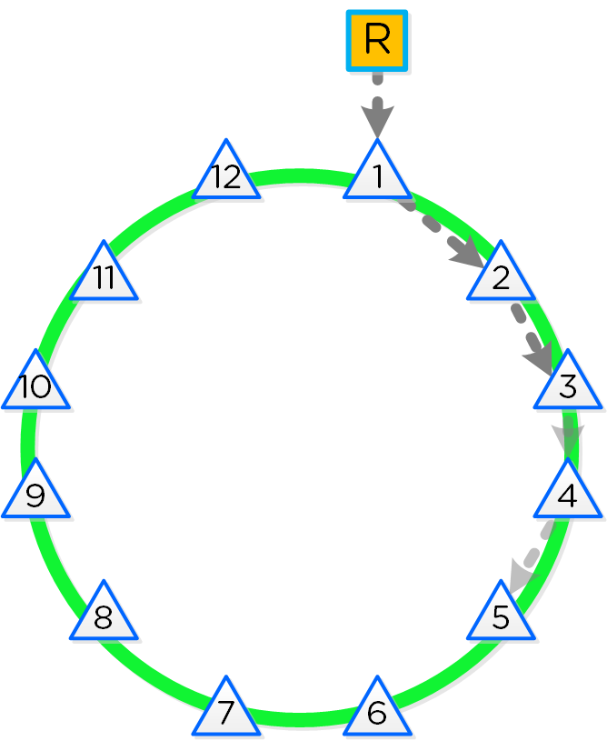12 Node Cassandra Ring

Cassandra peer replication iterates through nodes in a clockwise manner throughout the ring. With [block/rack] awareness, the peers are distributed among the [blocks/racks] to ensure no two peers are on the same [block/rack].

The following figure shows an example node layout translating the ring above into the [block/rack] based layout:

Cassandra Node Block/Rack Aware Placement

With this [block/rack]-aware nature, in the event of a [block/rack] failure there will still be at least two copies of the data (with Metadata RF3 – In larger clusters RF5 can be leveraged).

The following figure shows an example of all of the nodes replication topology to form the ring (yes – it’s a little busy):

Full Cassandra Node Block/Rack Aware Placement

Configuration Data

Nutanix leverages Zookeeper to store essential configuration data for the cluster.  This role is also distributed in a [block/rack]-aware manner to ensure availability in the case of a [block/rack] failure.

The following figure shows an example layout showing 3 Zookeeper nodes distributed in a [block/rack]-aware manner:

Zookeeper Block/Rack Aware Placement

In the event of a [block/rack] outage, meaning one of the Zookeeper nodes will be gone, the Zookeeper role would be transferred to another node in the cluster as shown below:

Zookeeper Placement Block/Rack Failure

When the [block/rack] comes back online, the Zookeeper role would be transferred back to maintain [block/rack] awareness.

NOTE: Prior to 4.5, this migration was not automatic and must be done manually.

Data Path Resiliency

Reliability and resiliency are key, if not the most important concepts within AOS or any primary storage platform. 

Contrary to traditional architectures which are built around the idea that hardware will be reliable, Nutanix takes a different approach: it expects hardware will eventually fail.  By doing so, the system is designed to handle these failures in an elegant and non-disruptive manner.

NOTE: That doesn’t mean the hardware quality isn’t there, just a concept shift.  The Nutanix hardware and QA teams undergo an exhaustive qualification and vetting process.

As mentioned in the prior sections metadata and data are protected using a RF which is based upon the cluster FT level. As of 5.0 supported FT levels are FT1 and FT2 which correspond to metadata RF3 and data RF2, or metadata RF5 and data RF3 respectively.

To learn more about how metadata is sharded refer to the prior ‘Scalable Metadata’ section. To learn more about how data is protected refer to the prior ‘Data protection’ section.

In a normal state, cluster data layout will look similar to the following:

Data Path Resiliency - Normal State

As you can see the VM/vDisk data has 2 or 3 copies on disk which are distributed among the nodes and associated storage devices.

Potential levels of failure

Being a distributed system, AOS is built to handle component, service, and CVM failures, which can be characterized on a few levels:

• Disk Failure
• CVM “Failure”
• Node Failure

Disk Failure

A disk failure can be characterized as just that, a disk which has either been removed, encounters a failure, or one that is not responding or has I/O errors. When Stargate sees I/O errors or the device fails to respond within a certain threshold it will mark the disk offline. Once that has occurred Hades will run S.M.A.R.T. and check the status of the device. If the tests pass the disk will be marked online, if they fail it will remain offline. If Stargate marks a disk offline multiple times (currently 3 times in an hour), Hades will stop marking the disk online even if S.M.A.R.T. tests pass.

VM impact:

• HA event:No
• Failed I/Os:No
• Latency:No impact

In the event of a disk failure, a Curator scan (MapReduce Framework) will occur immediately.  It will scan the metadata (Cassandra) to find the data previously hosted on the failed disk and the nodes / disks hosting the replicas.

Once it has found that data that needs to be “re-replicated”, it will distribute the replication tasks to the nodes throughout the cluster. 

During this process a Drive Self Test (DST) is started for the bad disk and SMART logs are monitored for errors.

The following figure shows an example disk failure and re-protection:

Data Path Resiliency - Disk Failure

An important thing to highlight here is given how Nutanix distributes data and replicas across all nodes / CVMs / disks; all nodes / CVMs / disks will participate in the re-replication. 

This substantially reduces the time required for re-protection, as the power of the full cluster can be utilized; the larger the cluster, the faster the re-protection.

Node Failure

VM Impact:

• HA event:Yes
• Failed I/Os:No
• Latency:No impact

In the event of a node failure, a VM HA event will occur restarting the VMs on other nodes throughout the virtualization cluster.  Once restarted, the VMs will continue to perform I/Os as usual which will be handled by their local CVMs.

Similar to the case of a disk failure above, a Curator scan will find the data previously hosted on the node and its respective replicas. Once the replicas are found all nodes will participate in the reprotection.

Data Path Resiliency - Node Failure

In the event where the node remains down for a prolonged period of time (30 minutes as of 4.6), the down CVM will be removed from the metadata ring.  It will be joined back into the ring after it has been up and stable for a duration of time.

ncli cluster get-domain-fault-tolerance-status type=node

ncli cluster get-domain-fault-tolerance-status type=rackable_unit

CVM “Failure”

A CVM “failure” can be characterized as a CVM power action causing the CVM to be temporarily unavailable.  The system is designed to transparently handle these gracefully.  In the event of a failure, I/Os will be re-directed to other CVMs within the cluster.  The mechanism for this will vary by hypervisor. 

The rolling upgrade process actually leverages this capability as it will upgrade one CVM at a time, iterating through the cluster.

VM impact:

• HA event:No
• Failed I/Os:No
• Latency:Potentially higher given I/Os over the network

In the event of a CVM “failure” the I/O which was previously being served from the down CVM, will be forwarded to other CVMs throughout the cluster.  ESXi and Hyper-V handle this via a process called CVM Autopathing, which leverages HA.py (like “happy”), where it will modify the routes to forward traffic going to the internal address (192.168.5.2) to the external IP of other CVMs throughout the cluster.  This enables the datastore to remain intact, just the CVM responsible for serving the I/Os is remote.

Once the local CVM comes back up and is stable, the route would be removed and the local CVM would take over all new I/Os.

In the case of AHV, iSCSI multi-pathing is leveraged where the primary path is the local CVM and the two other paths would be remote.  In the event where the primary path fails, one of the other paths will become active.

Similar to Autopathing with ESXi and Hyper-V, when the local CVM comes back online, it’ll take over as the primary path.

Resilient Capacity

Some refresher on terms used:

• Failure/Availability Domain(FD): Logical grouping of entities across which replicas are placed. Node is default domain on Nutanix clusters for node sizes > 3. Refer to Availability Domain section.
• Replication Factor(RF): Number of copies of data to be maintained on cluster for data availability.
• Fault Tolerance(FT): Number of failure(s) of entities at configured FD that can be handled by cluster, ensuring data on failed entity is rebuilt completely.

Resilient capacity is storage capacity in a cluster that can be consumed at the lowest availability/failure domain while maintaining the cluster’s ability to self-heal and recover to desired replication factor (RF) after FT failure(s) at the configured availability/failure domain. So in simple terms, Resilient Capacity = Total Cluster Capacity - Capacity needed to rebuild from FT failure(s).

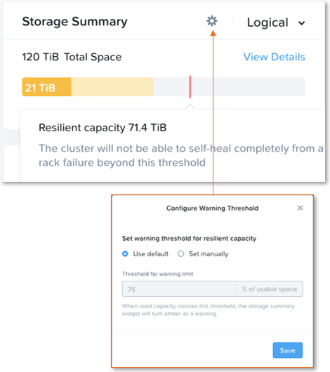
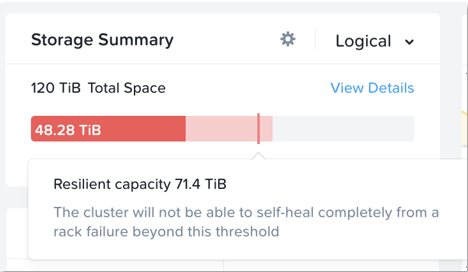
Starting with AOS 5.18, the resilient capacity is displayed in Prism Element storage summary widget with a gray line. Thresholds can be set to warn end users when cluster usage is reaching resilient capacity. By default that is set to 75%.

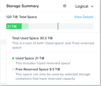
Prism can also show detailed storage utilizations on a per node basis which helps administrators understand resiliency on a per node basis. This is useful in clusters which have a skewed storage distribution.

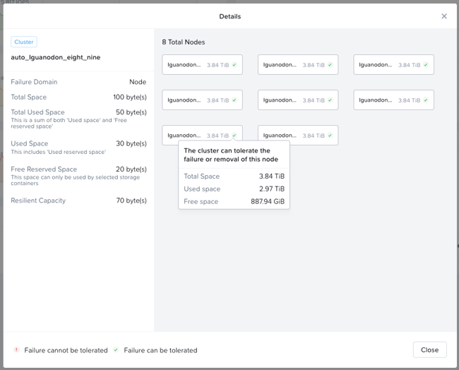
When cluster usage is greater than resilient capacity for that cluster, the cluster might not be able to tolerate and recover from failures anymore. Cluster can possibly still recover and tolerate failure at a lower failure domain as resilient capacity is for configured failure domain. For example, a cluster with a node failure domain may still be able to self-heal and recover from a disk failure but cannot self-heal and recover from a node failure.

It is highly recommeded to not exceed the resilient capacity of a cluster in any circumstances to ensure proper functioning of cluster and maintain it’s ability to self-heal and recover from failures.

Capacity Optimization

The Nutanix platform incorporates a wide range of storage optimization technologies that work in concert to make efficient use of available capacity for any workload. These technologies are intelligent and adaptive to workload characteristics, eliminating the need for manual configuration and fine-tuning.

The following optimizations are leveraged:

• Erasure Coding (EC-X)
• Compression
• Deduplication

More detail on how each of these features can be found in the following sections.

The table describes which optimizations are applicable to workloads at a high-level:

Erasure Coding

The Nutanix platform leverages a replication factor (RF) for data protection and availability.  This method provides the highest degree of availability because it does not require reading from more than one storage location or data re-computation on failure.  However, this does come at the cost of storage resources as full copies are required. 

To provide a balance between availability while reducing the amount of storage required, AOS provides the ability to encode data using erasure codes (EC).

Similar to the concept of RAID (levels 4, 5, 6, etc.) where parity is calculated, EC encodes a strip of data blocks on different nodes and calculates parity.  In the event of a host and/or disk failure, the parity can be leveraged to calculate any missing data blocks (decoding).  In the case of AOS, the data block is an extent group. Based upon the read nature of the data (read cold vs. read hot), the system will determine placement of the blocks in the strip.

For data that is read cold, we will prefer to distribute the data blocks from the same vDisk across nodes to form the strip (same-vDisk strip). This simplifies garbage collection (GC) as the full strip can be removed in the event the vDisk is deleted. For read hot data we will prefer to keep the vDisk data blocks local to the node and compose the strip with data from different vDisks (cross-vDisk strip). This minimizes remote reads as the local vDisk’s data blocks can be local and other VMs/vDisks can compose the other data blocks in the strip. In the event a read cold strip becomes hot, AOS will try to recompute the strip and localize the data blocks.

The number of data and parity blocks in a strip is configurable based upon the desired failures to tolerate.  The configuration is commonly referred to as the number of <number of data blocks>/<number of parity blocks>.

For example, “RF2 like” availability (N+1) could consist of 3 or 4 data blocks and 1 parity block in a strip (3/1 or 4/1).  “RF3 like” availability (N+2) could consist of 3 or 4 data blocks and 2 parity blocks in a strip (3/2 or 4/2). The default strip sizes are 4/1 for RF2 like availability and 4/2 for RF3 like availability. These can be overriden using nCLI is desired.

ncli container [create/edit] ... erasure-code=<N>/<K>

where N is number of data blocks and K is number of parity blocks

The expected overhead can be calculated as <# parity blocks> / <# data blocks>.  For example, a 4/1 strip has a 25% overhead or 1.25X compared to the 2X of RF2.  A 4/2 strip has a 50% overhead or 1.5X compared to the 3X of RF3.

The following table characterizes the encoded strip sizes and example overheads:

The encoding is done post-process and leverages the Curator MapReduce framework for task distribution. Since this is a post-process framework, the traditional write I/O path is unaffected.

A normal environment using RF would look like the following:

Typical AOS RF Data Layout

In this scenario, we have RF2 data whose primary copies are local and replicas are distributed to other nodes throughout the cluster.

When a Curator full scan runs, it will find eligible extent groups which are available to become encoded. Eligible extent groups must be “write-cold” meaning they haven’t been written to for awhile. This is controlled with the following Curator Gflag: curator_erasure_code_threshold_seconds. After the eligible candidates are found, the encoding tasks will be distributed and throttled via Chronos.

The following figure shows an example 3/1 strip:

AOS Encoded Strip - Pre-savings

Once the data has been successfully encoded (strips and parity calculation), the replica extent groups are then removed.

The following figure shows the environment after EC has run with the storage savings:

AOS Encoded Strip - Post-savings

Starting with AOS 5.18, inline erasure coding can be enabled on containers using nCLI. Inline erasure coding encodes and creates coding strips inline by erasure coding the data without waiting for it to become write-cold. In inline erasure coding, the erasure coded strips are created on the same vDisk data by default. With AOS 6.6 there is also an option to create strips from cross vdisks preserving data locality if that is desired. Due to this, it is only recommended for workloads that do not require data locality or perform numerous overwrites. Objects deployment have inline EC-X turned on by default.

Compression

For a visual explanation, you can watch the following video: LINK

The Nutanix Capacity Optimization Engine (COE) is responsible for performing data transformations to increase data efficiency on disk.  Currently compression is one of the key features of the COE to perform data optimization. AOS provides both inline and offline flavors of compression to best suit the customer’s needs and type of data. As of 5.1, offline compression is enabled by default.

Inline compression will compress sequential streams of data or large I/O sizes (>64K) when written to the Extent Store (SSD + HDD). This includes data draining from OpLog as well as sequential data skipping it.

Offline compression will initially write the data as normal (in an un-compressed state) and then leverage the Curator framework to compress the data cluster wide. When inline compression is enabled but the I/Os are random in nature, the data will be written un-compressed in the OpLog, coalesced, and then compressed in memory before being written to the Extent Store.

Nutanix leverages LZ4 and LZ4HC for data compression with AOS 5.0 and beyond. Prior to AOS 5.0 the Google Snappy compression library is leveraged which provides good compression ratios with minimal computational overhead and extremely fast compression / decompression rates.

Normal data will be compressed using LZ4 which provides a very good blend between compression and performance. For cold data, LZ4HC will be leveraged to provide an improved compression ratio.

Cold data is characterized into two main categories:

• Regular data: No R/W access for 3 days (Gflag: curator_medium_compress_mutable_data_delay_secs)
• Immutable data (snapshots): No R/W access for 1 day (Gflag: curator_medium_compress_immutable_data_delay_secs)

The following figure shows an example of how inline compression interacts with the AOS write I/O path:

Inline Compression I/O Path

For offline compression, all new write I/O is written in an un-compressed state and follows the normal AOS I/O path.  After the compression delay (configurable) is met, the data is eligible to become compressed. Compression can occur anywhere in the Extent Store. Offline compression uses the Curator MapReduce framework and all nodes will perform compression tasks.  Compression tasks will be throttled by Chronos.

The following figure shows an example of how offline compression interacts with the AOS write I/O path:

Offline Compression I/O Path

For read I/O, the data is first decompressed in memory and then the I/O is served.

You can view the current compression rates via Prism on the Storage > Dashboard page.

Elastic Dedupe Engine

For a visual explanation, you can watch the following video: LINK

The Elastic Dedupe Engine is a software-based feature of AOS which allows for data deduplication in the capacity (Extent Store) tiers.  Streams of data are fingerprinted during ingest at a 16KB granularity (Controlled by: stargate_dedup_fingerprint) within a 1MB extent. Prior to AOS 5.11, AOS used only SHA-1 hash to fingerprint and identify candidates for dedupe. Since AOS 5.11, AOS now uses logical checksums to select candidates for dedupe. This fingerprint is only done on data ingest and is then stored persistently as part of the written block’s metadata.

Contrary to traditional approaches which utilize background scans requiring the data to be re-read, Nutanix performs the fingerprint inline on ingest.  For duplicate data that can be deduplicated in the capacity tier, the data does not need to be scanned or re-read, essentially duplicate copies can be removed.

To make the metadata overhead more efficient, fingerprint refcounts are monitored to track dedupability. Fingerprints with low refcounts will be discarded to minimize the metadata overhead. To minimize fragmentation full extents will be preferred for deduplication.

Fingerprinting is done during data ingest of data with an I/O size of 64K or greater (initial I/O or when draining from OpLog). AOS then looks at hashes/fingerprints of each 16KB chunk within a 1MB extent and if it finds duplicates for more than 40% of chunks, it dedupes the entire extent. That resulted in many dedupe extents with reference count of 1 (no other duplicates) within the 1MB extent from the remaining 60% of extent, that ended up using metadata.

With AOS 6.6, the algorithm was further enhanced such that within a 1MB extent, only chunks that have duplicates will be marked for deduplication instead of entire extent reducing the metadata required. With AOS 6.6, changes were also made with the way dedupe metadata was stored. Before AOS 6.6, dedupe metadata was stored in a top level vdisk block map which resulted in dedupe metadata to be copied when snapshots were taken. This resulted in a metadata bloat. With AOS 6.6, that metadata is now stored in extent group id map which is a level lower than vdisk block map. Now when snapshots are taken of the vdisk, it does not result in copying of dedupe metadata and prevents metadata bloat. Once the fingerprintng is done, a background process will remove the duplicate data using the AOS MapReduce framework (Curator). For data that is being read, the data will be pulled into the AOS Unified Cache which is a multi-tier/pool cache.  Any subsequent requests for data having the same fingerprint will be pulled directly from the cache.  To learn more about the Unified Cache and pool structure, please refer to the Unified Cache sub-section in the I/O path overview.

The following figure shows an example of how the Elastic Dedupe Engine interacts with the AOS I/O path:

EDE I/O Path

You can view the current deduplication rates via Prism on the Storage > Dashboard page.

Storage Tiering and Prioritization

The Disk Balancing section below talks about how storage capacity was pooled among all nodes in a Nutanix cluster and that ILM would be used to keep hot data local.  A similar concept applies to disk tiering, in which the cluster’s SSD and HDD tiers are cluster-wide and AOS ILM is responsible for triggering data movement events. A local node’s SSD tier is always the highest priority tier for all I/O generated by VMs running on that node, however all of the cluster’s SSD resources are made available to all nodes within the cluster.  The SSD tier will always offer the highest performance and is a very important thing to manage for hybrid arrays.

The tier prioritization can be classified at a high-level by the following:

AOS Tier Prioritization

Specific types of resources (e.g. SSD, HDD, etc.) are pooled together and form a cluster wide storage tier.  This means that any node within the cluster can leverage the full tier capacity, regardless if it is local or not.

The following figure shows a high level example of what this pooled tiering looks like:

AOS Cluster-wide Tiering

A common question is what happens when a local node’s SSD becomes full?  As mentioned in the Disk Balancing section, a key concept is trying to keep uniform utilization of devices within disk tiers.  In the case where a local node’s SSD utilization is high, disk balancing will kick in to move the coldest data on the local SSDs to the other SSDs throughout the cluster.  This will free up space on the local SSD to allow the local node to write to SSD locally instead of going over the network.  A key point to mention is that all CVMs and SSDs are used for this remote I/O to eliminate any potential bottlenecks and remediate some of the hit by performing I/O over the network.

AOS Cluster-wide Tier Balancing

The other case is when the overall tier utilization breaches a specific threshold [curator_tier_usage_ilm_threshold_percent (Default=75)] where AOS ILM will kick in and as part of a Curator job will down-migrate data from the SSD tier to the HDD tier.  This will bring utilization within the threshold mentioned above or free up space by the following amount [curator_tier_free_up_percent_by_ilm (Default=15)], whichever is greater. The data for down-migration is chosen using last access time. In the case where the SSD tier utilization is 95%, 20% of the data in the SSD tier will be moved to the HDD tier (95% –> 75%). 

However, if the utilization was 80%, only 15% of the data would be moved to the HDD tier using the minimum tier free up amount.

AOS Tier ILM

AOS ILM will constantly monitor the I/O patterns and (down/up) migrate data as necessary as well as bring the hottest data local regardless of tier. The logic for up-migration (or horizontal) follows the same as that defined for egroup locality: “3 touches for random or 10 touches for sequential within a 10 minute window where multiple reads every 10 second sampling count as a single touch”.

Disk Balancing

For a visual explanation, you can watch the following video: LINK

AOS is designed to be a very dynamic platform which can react to various workloads as well as allow heterogeneous node types: compute heavy (3050, etc.) and storage heavy (60X0, etc.) to be mixed in a single cluster.  Ensuring uniform distribution of data is an important item when mixing nodes with larger storage capacities. AOS has a native feature, called disk balancing, which is used to ensure uniform distribution of data throughout the cluster.  Disk balancing works on a node’s utilization of its local storage capacity and is integrated with AOS ILM.  Its goal is to keep utilization uniform among nodes once the utilization has breached a certain threshold.

NOTE: Disk balancing jobs are handled by Curator which has different priority queues for primary I/O (UVM I/O) and background I/O (e.g. disk balancing). This is done to ensure disk balancing or any other background activity doesn’t impact front-end latency / performance. In this cases the job’s tasks will be given to Chronos who will throttle / control the execution of the tasks. Also, movement is done within the same tier for disk balancing. For example, if data is skewed in the HDD tier, it can be moved amongst nodes in the same tier.

The following figure shows an example of a mixed cluster (3050 + 6050) in an “unbalanced” state:

Disk Balancing - Unbalanced State

Disk balancing leverages the AOS Curator framework and is run as a scheduled process as well as when a threshold has been breached (e.g., local node capacity utilization > n %).  In the case where the data is not balanced, Curator will determine which data needs to be moved and will distribute the tasks to nodes in the cluster. In the case where the node types are homogeneous (e.g., 3050), utilization should be fairly uniform. However, if there are certain VMs running on a node which are writing much more data than others, this can result in a skew in the per node capacity utilization.  In this case, disk balancing would run and move the coldest data on that node to other nodes in the cluster. In the case where the node types are heterogeneous (e.g., 3050 + 6020/50/70), or where a node may be used in a “storage only” mode (not running any VMs), there will likely be a requirement to move data.

The following figure shows an example the mixed cluster after disk balancing has been run in a “balanced” state:

Disk Balancing - Balanced State

In some scenarios, customers might run some nodes in a “storage-only” state where only the CVM will run on the node whose primary purpose is bulk storage capacity.  In this case, the full node’s memory can be added to the CVM to provide a much larger read cache.

The following figure shows an example of how a storage only node would look in a mixed cluster with disk balancing moving data to it from the active VM nodes:

Disk Balancing - Storage Only Node

Snapshots and Clones

For a visual explanation, you can watch the following video: LINK

AOS provides native support for offloaded snapshots and clones which can be leveraged via VAAI, ODX, ncli, REST, Prism, etc.  Both the snapshots and clones leverage the redirect-on-write algorithm which is the most effective and efficient. As explained in the Data Structure section above, a virtual machine consists of files (vmdk/vhdx) which are vDisks on the Nutanix platform. 

A vDisk is composed of extents which are logically contiguous chunks of data, which are stored within extent groups which are physically contiguous data stored as files on the storage devices. When a snapshot or clone is taken, the base vDisk is marked immutable and another vDisk is created as read/write.  At this point, both vDisks have the same block map, which is a metadata mapping of the vDisk to its corresponding extents. Contrary to traditional approaches which require traversal of the snapshot chain (which can add read latency), each vDisk has its own block map.  This eliminates any of the overhead normally seen by large snapshot chain depths and allows you to take continuous snapshots without any performance impact.

The following figure shows an example of how this works when a snapshot is taken (source: NTAP):

Example Snapshot Block Map

The same method applies when a snapshot or clone of a previously snapped or cloned vDisk is performed:

Multi-snap Block Map and New Write

The same methods are used for both snapshots and/or clones of a VM or vDisk(s).  When a VM or vDisk is cloned, the current block map is locked and the clones are created.  These updates are metadata only, so no I/O actually takes place.  The same method applies for clones of clones; essentially the previously cloned VM acts as the “Base vDisk” and upon cloning, that block map is locked and two “clones” are created: one for the VM being cloned and another for the new clone.  There is no imposed limit on the maximum number of clones.

They both inherit the prior block map and any new writes/updates would take place on their individual block maps.

Multi-Clone Block Maps

As mentioned previously, each VM/vDisk has its own individual block map.  So in the above example, all of the clones from the base VM would now own their block map and any write/update would occur there.

In the event of an overwrite the data will go to a new extent / extent group. For example, if data exists at offset o1 in extent e1 that was being overwritten, Stargate would create a new extent e2 and track that the new data was written in extent e2 at offset o2. The Vblock map tracks this down to the byte level.

The following figure shows an example of what this looks like:

Clone Block Maps - New Write

Any subsequent clones or snapshots of a VM/vDisk would cause the original block map to be locked and would create a new one for R/W access.

Networking and I/O

The Nutanix platform does not leverage any backplane for inter-node communication and only relies on a standard 10GbE network.  All storage I/O for VMs running on a Nutanix node is handled by the hypervisor on a dedicated private network.  The I/O request will be handled by the hypervisor, which will then forward the request to the private IP on the local CVM.  The CVM will then perform the remote replication with other Nutanix nodes using its external IP over the public 10GbE network. For all read requests, these will be served completely locally in most cases and never touch the 10GbE network. This means that the only traffic touching the public 10GbE network will be AOS remote replication traffic and VM network I/O.  There will, however, be cases where the CVM will forward requests to other CVMs in the cluster in the case of a CVM being down or data being remote.  Also, cluster-wide tasks, such as disk balancing, will temporarily generate I/O on the 10GbE network.

The following figure shows an example of how the VM’s I/O path interacts with the private and public 10GbE network:

AOS Networking

Data Locality

Being a converged (compute+storage) platform, I/O and data locality are critical to cluster and VM performance with Nutanix.  As explained above in the I/O path, all read/write IOs are served by the local Controller VM (CVM) which is on each hypervisor adjacent to normal VMs.  A VM’s data is served locally from the CVM and sits on local disks under the CVM’s control.  When a VM is moved from one hypervisor node to another (or during a HA event), the newly migrated VM’s data will be served by the now local CVM. When reading old data (stored on the now remote node/CVM), the I/O will be forwarded by the local CVM to the remote CVM.  All write I/Os will occur locally right away.  AOS will detect the I/Os are occurring from a different node and will migrate the data locally in the background, allowing for all read I/Os to now be served locally.  The data will only be migrated on a read as to not flood the network.

Data locality occurs in two main flavors:

• Cache Locality
  • Pulling remote data into the local Stargate’s Unified Cache. This is done at a 4K granularity.
  • For instances where there are no local replicas, the requests will be forward to the Stargate(s) containing the replicas which will return the data and the local Stargate will store this locally then return the I/O. All subsequent requests for that data will be returned from the cache.
• Extent Group (egroup) Locality
  • Migrating the vDisk extent group(s) (egroups) to be stored in the local Stargate’s Extent Store.
  • If a replica egroup is already local, no movement is necessary.
  • In this scenario the actual replica egroup will be re-localized after certain I/O thresholds are met. We don’t automatically re-localize / migrate egroups to ensure we’re leveraging the network efficiently.
  • For AES enabled egroups the same horizontal migration occurs for cases where replicas aren’t local and the patterns are met.

The following figure shows an example of how data will “follow” the VM as it moves between hypervisor nodes:

Data Locality

Shadow Clones

The Distributed Storage Fabric has a feature called ‘Shadow Clones’, which allows for distributed caching of particular vDisks or VM data which is in a ‘multi-reader’ scenario.  A great example of this is during a VDI deployment many ‘linked clones’ will be forwarding read requests to a central master or ‘Base VM’.  In the case of VMware View, this is called the replica disk and is read by all linked clones, and in XenDesktop, this is called the MCS Master VM.  This will also work in any scenario which may be a multi-reader scenario (e.g., deployment servers, repositories, etc.). Data or I/O locality is critical for the highest possible VM performance and a key struct of AOS. 

With Shadow Clones, AOS will monitor vDisk access trends similar to what it does for data locality.  However, in the case there are requests occurring from more than two remote CVMs (as well as the local CVM), and all of the requests are read I/O, the vDisk will be marked as immutable.  Once the disk has been marked as immutable, the vDisk can then be cached locally by each CVM making read requests to it (aka Shadow Clones of the base vDisk). This will allow VMs on each node to read the Base VM’s vDisk locally. In the case of VDI, this means the replica disk can be cached by each node and all read requests for the base will be served locally.  NOTE:  The data will only be migrated on a read as to not flood the network and allow for efficient cache utilization.  In the case where the Base VM is modified, the Shadow Clones will be dropped and the process will start over.  Shadow clones are enabled by default (as of 4.0.2) and can be enabled/disabled using the following NCLI command: ncli cluster edit-params enable-shadow-clones=<true/false>.

The following figure shows an example of how Shadow Clones work and allow for distributed caching:

Shadow Clones

Storage Layers and Monitoring

The Nutanix platform monitors storage at multiple layers throughout the stack, ranging from the VM/Guest OS all the way down to the physical disk devices.  Knowing the various tiers and how these relate is important whenever monitoring the solution and allows you to get full visibility of how the ops relate. The following figure shows the various layers of where operations are monitored and the relative granularity which are explained below:

Storage Layers

Virtual Machine Layer

• Key Role: Metrics reported by the hypervisor for the VM
• Description: Virtual Machine or guest level metrics are pulled directly from the hypervisor and represent the performance the VM is seeing and is indicative of the I/O performance the application is seeing.
• When to use: When troubleshooting or looking for VM level detail

Hypervisor Layer

• Key Role: Metrics reported by the Hypervisor(s)
• Description: Hypervisor level metrics are pulled directly from the hypervisor and represent the most accurate metrics the hypervisor(s) are seeing. This data can be viewed for one of more hypervisor node(s) or the aggregate cluster. This layer will provide the most accurate data in terms of what performance the platform is seeing and should be leveraged in most cases. In certain scenarios the hypervisor may combine or split operations coming from VMs which can show the difference in metrics reported by the VM and hypervisor. These numbers will also include cache hits served by the Nutanix CVMs.
• When to use: Most common cases as this will provide the most detailed and valuable metrics.

Controller Layer

• Key Role: Metrics reported by the Nutanix Controller(s)
• Description: Controller level metrics are pulled directly from the Nutanix Controller VMs (e.g., Stargate 2009 page) and represent what the Nutanix front-end is seeing from NFS/SMB/iSCSI or any back-end operations (e.g., ILM, disk balancing, etc.). This data can be viewed for one of more Controller VM(s) or the aggregate cluster. The metrics seen by the Controller Layer should normally match those seen by the hypervisor layer, however will include any backend operations (e.g., ILM, disk balancing). These numbers will also include cache hits served by memory. In certain cases, metrics like (IOPS), might not match as the NFS / SMB / iSCSI client might split a large IO into multiple smaller IOPS. However, metrics like bandwidth should match.
• When to use: Similar to the hypervisor layer, can be used to show how much backend operation is taking place.

Disk Layer

• Key Role: Metrics reported by the Disk Device(s)
• Description: Disk level metrics are pulled directly from the physical disk devices (via the CVM) and represent what the back-end is seeing. This includes data hitting the OpLog or Extent Store where an I/O is performed on the disk. This data can be viewed for one of more disk(s), the disk(s) for a particular node, or the aggregate disks in the cluster. In common cases, it is expected that the disk ops should match the number of incoming writes as well as reads not served from the memory portion of the cache. Any reads being served by the memory portion of the cache will not be counted here as the op is not hitting the disk device.
• When to use: When looking to see how many ops are served from cache or hitting the disks.